Withdrawal prediction on behavioral indicators#
In this section, we try to reproduce the withdrawal prediction approach based on behavioral indicators and Synthetic Minority Over-sampling (SMOTE) as presented in the work of Hlioui et al. [HAG21].
Given the recurring occurrence of elevated learner withdrawal rates in Massive Open Online Courses (MOOCs), the implementation of early withdrawal prediction models could facilitate pedagogical enhancements, enable tailored intervention strategies and empower learners to monitor and enhance their academic performance.
The approach of Hlioui et al. encloses four main phases:
Data preprocessing
Behavioral indicators extraction (feature engineering)
K-means-based Data Discretizing
Withdrawal prediction
Fedia Hlioui, Nadia Aloui, and Faiez Gargouri. A withdrawal prediction model of at-risk learners based on behavioural indicators. International Journal of Web-Based Learning and Teaching Technologies, 16(2):32–53, 2021. doi:10.4018/ijwltt.2021030103.
from itertools import chain

import pandas as pd
from imblearn.over_sampling import SMOTE
from IPython.display import display
from matplotlib import pyplot as plt
from sklearn.cluster import KMeans
from sklearn.ensemble import RandomForestClassifier
from sklearn.model_selection import GridSearchCV, StratifiedKFold, train_test_split
from sklearn.naive_bayes import GaussianNB
from sklearn.neural_network import MLPClassifier
from sklearn.preprocessing import MinMaxScaler, OrdinalEncoder
from sklearn.svm import SVC
from sklearn.tree import DecisionTreeClassifier

from oulad import filter_by_module_presentation, get_oulad

%load_ext oulad.capture
%%capture oulad
oulad = get_oulad()
Data preprocessing#
As in the work of Hlioui et al., we use the data from the DDD course 2013B
presentation.
We start by extracting three tables containing data related to student demographics,
student assessments and student course interactions.
MODULE = "DDD"
PRESENTATION = "2013B"
Student demographics table#
student_info = filter_by_module_presentation(
    oulad.student_info, MODULE, PRESENTATION
).drop(columns=["studied_credits", "imd_band"])
display(student_info)
| id_student | gender | region | highest_education | age_band | num_of_prev_attempts | disability | final_result | |
|---|---|---|---|---|---|---|---|---|
| 13091 | 24213 | F | East Anglian Region | A Level or Equivalent | 0-35 | 0 | N | Withdrawn |
| 13092 | 40419 | M | East Midlands Region | Lower Than A Level | 35-55 | 0 | N | Withdrawn |
| 13093 | 41060 | M | Ireland | HE Qualification | 0-35 | 0 | N | Fail |
| 13094 | 43284 | M | East Midlands Region | Lower Than A Level | 0-35 | 2 | N | Withdrawn |
| 13095 | 45664 | M | Yorkshire Region | HE Qualification | 0-35 | 1 | N | Pass |
| ... | ... | ... | ... | ... | ... | ... | ... | ... |
| 14389 | 2693243 | F | Yorkshire Region | Lower Than A Level | 35-55 | 0 | N | Distinction |
| 14390 | 2694933 | F | East Midlands Region | A Level or Equivalent | 0-35 | 0 | Y | Pass |
| 14391 | 2697773 | F | East Anglian Region | A Level or Equivalent | 0-35 | 0 | N | Fail |
| 14392 | 2707979 | F | East Midlands Region | Lower Than A Level | 0-35 | 0 | N | Fail |
| 14393 | 2710343 | M | North Western Region | Lower Than A Level | 0-35 | 0 | N | Fail |
1303 rows × 8 columns
Student assessments table#
assessments = filter_by_module_presentation(oulad.assessments, MODULE, PRESENTATION)
student_assessments = assessments.merge(
    oulad.student_assessment, on="id_assessment"
).drop(columns=["is_banked", "assessment_type", "id_assessment"])
display(student_assessments)
| date | weight | id_student | date_submitted | score | |
|---|---|---|---|---|---|
| 0 | 23.0 | 2.0 | 907261 | 25 | 80.0 |
| 1 | 23.0 | 2.0 | 957467 | 25 | 77.0 |
| 2 | 23.0 | 2.0 | 1018685 | 25 | 40.0 |
| 3 | 23.0 | 2.0 | 1044992 | 25 | 73.0 |
| 4 | 23.0 | 2.0 | 1068316 | 25 | 67.0 |
| ... | ... | ... | ... | ... | ... |
| 10368 | 240.0 | 100.0 | 2677955 | 230 | 69.0 |
| 10369 | 240.0 | 100.0 | 2683836 | 230 | 71.0 |
| 10370 | 240.0 | 100.0 | 2689536 | 229 | 58.0 |
| 10371 | 240.0 | 100.0 | 2693243 | 230 | 82.0 |
| 10372 | 240.0 | 100.0 | 2694933 | 230 | 73.0 |
10373 rows × 5 columns
Student course interactions table#
%%capture -ns withdrawal_prediction_on_behavioral_indicators student_vle
student_vle = (
    filter_by_module_presentation(oulad.student_vle, MODULE, PRESENTATION)
    .merge(filter_by_module_presentation(oulad.vle, MODULE, PRESENTATION), on="id_site")
    .drop(columns=["id_site", "date", "week_from", "week_to"])
)
display(student_vle)
| id_student | sum_click | activity_type | |
|---|---|---|---|
| 0 | 430516 | 3 | page |
| 1 | 430516 | 6 | homepage |
| 2 | 430516 | 2 | url |
| 3 | 420388 | 1 | url |
| 4 | 420388 | 3 | homepage |
| ... | ... | ... | ... |
| 536832 | 536170 | 2 | resource |
| 536833 | 536926 | 1 | homepage |
| 536834 | 556295 | 3 | homepage |
| 536835 | 556780 | 1 | homepage |
| 536836 | 556918 | 2 | homepage |
536837 rows × 3 columns
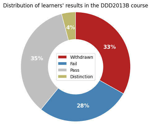
Distribution of learners’ results in the course DDD2013B#
Next, we reproduce the pie chart from the paper of Hlioui et al. (Figure 3)
which reveals class imbalance of student final outcome in the DDD2013B course
presentation.
The class imbalance problem is a commonly recognized challenge in Machine Learning, known to hinder the development of effective classifiers. (Batista, et al., 2004)
When trained on imbalanced datasets, models often exhibit a significant bias toward the majority class. This bias occurs because traditional Machine Learning algorithms are primarily focused on maximizing overall prediction accuracy, which can lead them to overlook or neglect classes with fewer instances, typically referred to as the minority class. (Bekkar & Alitouche, 2013)
To deal with the class imbalance problem, the approach of Hlioui et al. applies the Synthetic Minority Over-sampling method (SMOTE) on the dataset, which generates new observations in the minority class by interpolating the existing ones.
Note
At this juncture, we deviate marginally from the initial approach as we apply the SMOTE method subsequent to the extraction of behavioral indicators.
(
    student_info.final_result.value_counts()
    .loc[["Withdrawn", "Fail", "Pass", "Distinction"]]
    .plot.pie(
        title="Distribution of learners' results in the DDD2013B course",
        ylabel="",
        wedgeprops={"width": 0.6, "edgecolor": "w"},
        autopct="%1.0f%%",
        pctdistance=0.72,
        colors=["firebrick", "steelblue", "silver", "darkkhaki"],
        startangle=-270,
        counterclock=False,
        labeldistance=None,
        radius=1.2,
        textprops={"color": "white", "weight": "bold", "fontsize": 12.5},
    )
)
plt.legend(loc="center")
plt.show()
Behavioral indicators extraction#
At this stage we extract behavioral indicators as described in the work of Hlioui et al.
Autonomy#
The autonomy indicator refers to the navigation frequency of learners within the virtual learning environment (VLE).
autonomy = (
    student_vle.drop(columns="activity_type")
    .groupby(["id_student"])
    .count()
    .rename(columns={"sum_click": "autonomy"})
)
display(autonomy)
| autonomy | |
|---|---|
| id_student | |
| 40419 | 60 |
| 41060 | 214 |
| 43284 | 422 |
| 45664 | 405 |
| 52014 | 116 |
| ... | ... |
| 2691780 | 156 |
| 2692101 | 151 |
| 2693243 | 1249 |
| 2694933 | 398 |
| 2697773 | 86 |
1214 rows × 1 columns
Perseverance#
The perseverance indicator refers to the ratio of evaluations submitted on time by the learners.
perseverance = (
    student_assessments.query("date_submitted <= date")[["id_student", "score"]]
    .groupby("id_student")
    .count()
    .div(assessments.shape[0])
    .rename(columns={"score": "perseverance"})
)
display(perseverance)
| perseverance | |
|---|---|
| id_student | |
| 40419 | 0.071429 |
| 41060 | 0.357143 |
| 43284 | 0.214286 |
| 45664 | 0.500000 |
| 52014 | 0.357143 |
| ... | ... |
| 2689536 | 0.285714 |
| 2691780 | 0.214286 |
| 2692101 | 0.071429 |
| 2693243 | 0.500000 |
| 2694933 | 0.428571 |
969 rows × 1 columns
Commitment indicators#
Commitment indicators aim to measure the level and type of involvement of learners. In the work of Hlioui et al. they refer to the total sum of clicks (interactions) made by learners on several related activity types (activity categories).
Below, a barplot is presented, illustrating the frequency distribution of interactions by activity type within the DDD2013B course.
student_vle.activity_type.value_counts().to_frame().plot.barh(
    title="Activity type frequency in the DDD2013B course", xlabel="Frequency"
)
plt.show()

Collaborative commitment#
The collaborative commitment indicator refers to the sum of clicks learners made on
activities of type forumng, ouwiki, and ouelluminate.
collaborative_commitment = (
    student_vle.query("activity_type in ['forumng', 'ouwiki', 'ouelluminate']")
    .drop(columns="activity_type")
    .groupby("id_student")
    .sum()
    .rename(columns={"sum_click": "collaborative_commitment"})
)
display(collaborative_commitment)
| collaborative_commitment | |
|---|---|
| id_student | |
| 40419 | 69 |
| 41060 | 46 |
| 43284 | 176 |
| 45664 | 181 |
| 52014 | 110 |
| ... | ... |
| 2691780 | 43 |
| 2692101 | 32 |
| 2693243 | 941 |
| 2694933 | 305 |
| 2697773 | 32 |
1106 rows × 1 columns
Course structure commitment#
The course structure commitment indicator refers to the sum of clicks learners made on
activities of type homepage and glossary.
course_structure_commitment = (
    student_vle.query("activity_type in ['homepage', 'glossary']")
    .drop(columns="activity_type")
    .groupby("id_student")
    .sum()
    .rename(columns={"sum_click": "course_structure_commitment"})
)
display(course_structure_commitment)
| course_structure_commitment | |
|---|---|
| id_student | |
| 40419 | 29 |
| 41060 | 80 |
| 43284 | 293 |
| 45664 | 287 |
| 52014 | 98 |
| ... | ... |
| 2691780 | 87 |
| 2692101 | 69 |
| 2693243 | 591 |
| 2694933 | 279 |
| 2697773 | 37 |
1211 rows × 1 columns
Course content commitment#
The course content commitment indicator refers to the sum of clicks learners made on
activities of type resource, url, oucontent, page, and subpage.
course_content_commitment = (
    student_vle.query(
        "activity_type in ['resource', 'url', 'oucontent', 'page', 'subpage']"
    )
    .drop(columns="activity_type")
    .groupby("id_student")
    .sum()
    .rename(columns={"sum_click": "course_content_commitment"})
)
display(course_content_commitment)
| course_content_commitment | |
|---|---|
| id_student | |
| 40419 | 45 |
| 41060 | 270 |
| 43284 | 348 |
| 45664 | 558 |
| 52014 | 132 |
| ... | ... |
| 2691780 | 154 |
| 2692101 | 215 |
| 2693243 | 1050 |
| 2694933 | 310 |
| 2697773 | 79 |
1206 rows × 1 columns
Evaluation activities commitment#
The evaluation activities commitment indicator refers to the sum of clicks learners
made on activities of type extenalquiz.
evalutation_activities_commitment = (
    student_vle.query("activity_type == 'externalquiz'")
    .drop(columns="activity_type")
    .groupby("id_student")
    .sum()
    .rename(columns={"sum_click": "evalutation_activities_commitment"})
)
display(evalutation_activities_commitment)
| evalutation_activities_commitment | |
|---|---|
| id_student | |
| 40419 | 1 |
| 41060 | 15 |
| 43284 | 30 |
| 45664 | 22 |
| 52014 | 9 |
| ... | ... |
| 2689536 | 8 |
| 2691780 | 24 |
| 2692101 | 2 |
| 2693243 | 61 |
| 2694933 | 41 |
1103 rows × 1 columns
Motivation#
The motivation indicator measures whether a learners’ sum of clicks on all activities is above average (motivated) or below (unmotivated).
motivation = (
    student_vle.drop(columns="activity_type")
    .groupby("id_student")
    .sum()
    .assign(motivation=lambda df: df.sum_click >= df.sum_click.mean())
    .drop(columns="sum_click")
    .astype(float)
)
display(motivation)
| motivation | |
|---|---|
| id_student | |
| 40419 | 0.0 |
| 41060 | 0.0 |
| 43284 | 0.0 |
| 45664 | 0.0 |
| 52014 | 0.0 |
| ... | ... |
| 2691780 | 0.0 |
| 2692101 | 0.0 |
| 2693243 | 1.0 |
| 2694933 | 0.0 |
| 2697773 | 0.0 |
1214 rows × 1 columns
Performance#
The performance indicator refers to the sum of weighted assessment scores by learner.
performance = (
    student_assessments.assign(performance=lambda df: df.weight * df.score)
    .drop(columns=["date", "date_submitted", "weight", "score"])
    .groupby("id_student")
    .sum()
)
display(performance)
| performance | |
|---|---|
| id_student | |
| 40419 | 704.0 |
| 41060 | 6359.5 |
| 43284 | 4020.0 |
| 45664 | 9528.0 |
| 52014 | 4424.0 |
| ... | ... |
| 2689536 | 10621.0 |
| 2691780 | 2703.0 |
| 2692101 | 1819.0 |
| 2693243 | 17058.0 |
| 2694933 | 14997.0 |
1065 rows × 1 columns
K-Means-based data discretizing#
At this stage, we discretize the generated indicators using the K-Means clustering method. We begin by estimating the ‘k’ parameter through the elbow method and then replace the indicators’ values with their corresponding clustering labels.
Elbow method#
%%capture -ns withdrawal_prediction_on_behavioral_indicators inertia
indicators = {
    "Perseverance indicator": perseverance,
    "Autonomy indicator": autonomy,
    "Structure content commitment indicator": course_structure_commitment,
    "Evaluation activities commitment indicator": evalutation_activities_commitment,
    "Learning content commitment indicator": course_content_commitment,
    "Collaborative commitment indicator": collaborative_commitment,
    "Performance indicator": performance,
}
k_range = list(range(2, 10))
fig = plt.figure(figsize=(20, 20))
# Inertia: Sum of squared distances of samples to their closest cluster center,
# weighted by the sample weights if provided.
inertia = [
    KMeans(n_clusters=k, n_init="auto").fit(indicator.values).inertia_
    for indicator in indicators.values()
    for k in k_range
]
for i, name in enumerate(indicators):
    index = i * len(k_range)
    pd.Series(inertia[index : index + len(k_range)], index=k_range, name="k").plot(
        title=f"{name} (Inertia/k)",
        xlabel="Number of clusters",
        ylabel="SSE",
        grid=True,
        marker="s",
        ax=plt.subplot2grid((5, 5), (int(i / 2), 2 * (i % 2) + int(i / 6)), colspan=2),
    )

plt.subplots_adjust(hspace=0.4, wspace=0.4)
plt.show()
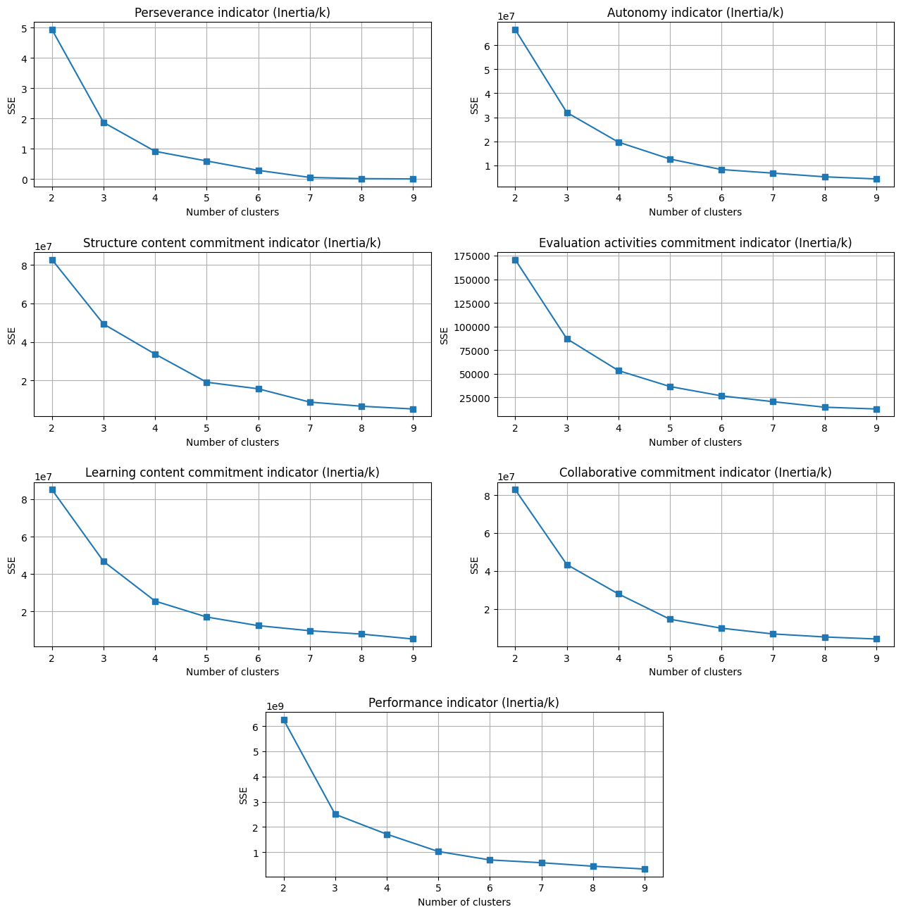
Discretization#
We obtain similar graphs as in the work of Hlioui et al.
Thus, we proceed by setting the same k values.
selected_k = {
    "Perseverance indicator": 3,
    "Autonomy indicator": 3,
    "Structure content commitment indicator": 2,
    "Evaluation activities commitment indicator": 3,
    "Learning content commitment indicator": 2,
    "Collaborative commitment indicator": 3,
    "Performance indicator": 3,
}
for name, k in selected_k.items():
    kmeans = KMeans(n_clusters=k, n_init="auto")
    indicator = indicators[name]
    indicator[indicator.columns[0]] = kmeans.fit_predict(indicator)
Feature table#
We join the student demographics table with the discretized behavioral
indicators into a single feature_table.
We also encode categorical columns (age_band, disability, gender,
highest_education, region, and final_result) to numerical values and fill
missing values with zeros.
region_encoder = OrdinalEncoder()
feature_table = (
    student_info.set_index("id_student")
    .join(chain([motivation], indicators.values()), how="outer")
    .fillna(0.0)
    .replace(
        {
            "age_band": {"0-35": "0.0", "35-55": "0.5", "55<=": "1.0"},
            "disability": {"N": "0.0", "Y": "1.0"},
            "gender": {"M": "0.0", "F": "1.0"},
            "highest_education": {
                "No Formal quals": "0.0",
                "Lower Than A Level": "0.25",
                "A Level or Equivalent": "0.5",
                "HE Qualification": "0.75",
                "Post Graduate Qualification": "1.0",
            },
            "final_result": {
                "Withdrawn": "1.0",
                "Fail": "0.0",
                "Pass": "0.0",
                "Distinction": "0.0",
            },
        }
    )
    .assign(region=lambda df: region_encoder.fit_transform(df[["region"]]))
    .astype(float)
)
display(feature_table)
| gender | region | highest_education | age_band | num_of_prev_attempts | disability | final_result | motivation | perseverance | autonomy | course_structure_commitment | evalutation_activities_commitment | course_content_commitment | collaborative_commitment | performance | |
|---|---|---|---|---|---|---|---|---|---|---|---|---|---|---|---|
| id_student | |||||||||||||||
| 24213 | 1.0 | 0.0 | 0.50 | 0.0 | 0.0 | 0.0 | 1.0 | 0.0 | 0.0 | 0.0 | 0.0 | 0.0 | 0.0 | 0.0 | 0.0 |
| 40419 | 0.0 | 1.0 | 0.25 | 0.5 | 0.0 | 0.0 | 1.0 | 0.0 | 1.0 | 0.0 | 0.0 | 0.0 | 1.0 | 0.0 | 0.0 |
| 41060 | 0.0 | 2.0 | 0.75 | 0.0 | 0.0 | 0.0 | 0.0 | 0.0 | 2.0 | 0.0 | 0.0 | 0.0 | 1.0 | 0.0 | 1.0 |
| 43284 | 0.0 | 1.0 | 0.25 | 0.0 | 2.0 | 0.0 | 1.0 | 0.0 | 1.0 | 1.0 | 0.0 | 1.0 | 1.0 | 0.0 | 0.0 |
| 45664 | 0.0 | 12.0 | 0.75 | 0.0 | 1.0 | 0.0 | 0.0 | 0.0 | 0.0 | 1.0 | 0.0 | 1.0 | 1.0 | 0.0 | 1.0 |
| ... | ... | ... | ... | ... | ... | ... | ... | ... | ... | ... | ... | ... | ... | ... | ... |
| 2693243 | 1.0 | 12.0 | 0.25 | 0.5 | 0.0 | 0.0 | 0.0 | 1.0 | 0.0 | 2.0 | 0.0 | 2.0 | 0.0 | 1.0 | 2.0 |
| 2694933 | 1.0 | 1.0 | 0.50 | 0.0 | 0.0 | 1.0 | 0.0 | 0.0 | 2.0 | 1.0 | 0.0 | 1.0 | 1.0 | 0.0 | 2.0 |
| 2697773 | 1.0 | 0.0 | 0.50 | 0.0 | 0.0 | 0.0 | 0.0 | 0.0 | 0.0 | 0.0 | 0.0 | 0.0 | 1.0 | 0.0 | 0.0 |
| 2707979 | 1.0 | 1.0 | 0.25 | 0.0 | 0.0 | 0.0 | 0.0 | 0.0 | 0.0 | 0.0 | 0.0 | 0.0 | 0.0 | 0.0 | 0.0 |
| 2710343 | 0.0 | 5.0 | 0.25 | 0.0 | 0.0 | 0.0 | 0.0 | 0.0 | 0.0 | 0.0 | 0.0 | 0.0 | 0.0 | 0.0 | 0.0 |
1303 rows × 15 columns
Withdrawal prediction#
Prior to training the classification models, we split the feature_table into a
train (75%) and test (25%) set.
Then we scale features to values between 0 and 1 and apply the SMOTE method to
balance the occurences of the target class (Withdrawn/Not Withdrawn).
x_train, x_test, y_train, y_test = train_test_split(
    feature_table.drop(columns="final_result").values, feature_table.final_result.values
)
scaler = MinMaxScaler()
x_train = scaler.fit_transform(x_train)
x_test = scaler.transform(x_test)
smote = SMOTE()
x_resampled, y_resampled = smote.fit_resample(x_train, y_train)
Subsequently, we undertake a grid search across classification parameters for five classifiers, which have been chosen to align closely with those utilized in the work of Hlioui et al. These classifiers encompass Decision Trees, Random Forest, Support Vector Machines, Gaussian Naive Bayes (as a substitute for Tree Augmented Naive Bayes), and Multilayer Perceptron.
In line with the work of Hlioui et al., we adopt a 5-fold cross-validation approach with stratification. Evaluation of classifier performance is conducted utilizing the F-measure as the primary metric.
Note
We replaced the initial parameter ranges with the selected values after the first grid search run to speed up the process.
%%capture -ns withdrawal_prediction_on_behavioral_indicators scores
grid = {
    DecisionTreeClassifier: {
        "unbalanced": {
            "criterion": ["log_loss"],  # ["gini", "entropy", "log_loss"],
            "max_depth": [3],  # [None, *list(range(1, 20))],
            "min_samples_leaf": [13],  # range(1, 20),
            "min_samples_split": [9],  # range(2, 20),
            "splitter": ["random"],  # ["random", "best"],
        },
        "balanced": {
            "criterion": ["entropy"],  # ["gini", "entropy", "log_loss"],
            "max_depth": [8],  # [None, *list(range(1, 20))],
            "min_samples_leaf": [1],  # range(1, 20),
            "min_samples_split": [12],  # range(2, 20),
            "splitter": ["random"],  # ["random", "best"],
        },
    },
    RandomForestClassifier: {
        "unbalanced": {
            "criterion": ["entropy"],  # ["gini", "entropy", "log_loss"],
            "max_depth": [15],  # [None, *list(range(1, 20, 2))],
            "min_samples_leaf": [3],  # list(range(1, 20, 2)),
            "min_samples_split": [2],  # list(range(2, 20, 2)),
            "n_estimators": [10],  # [10, 50, 100],
        },
        "balanced": {
            "criterion": ["entropy"],  # ["gini", "entropy", "log_loss"],
            "max_depth": [17],  # [None, *list(range(1, 20, 2))],
            "min_samples_leaf": [3],  # list(range(1, 20, 2)),
            "min_samples_split": [14],  # list(range(2, 20, 2)),
            "n_estimators": [50],  # [10, 50, 100],
        },
    },
    GaussianNB: {
        "unbalanced": {
            "var_smoothing": [0.001],  # [1/10**x for x in range(1, 11)],
        },
        "balanced": {
            "var_smoothing": [0.001],  # [1/10**x for x in range(1, 11)],
        },
    },
    SVC: {
        "unbalanced": {
            "C": [1.0],  # [1.0],
            "gamma": [0.5],  # ["scale", "auto", 0, 0.5],
            "kernel": ["poly"],  # ["rbf", "poly", "sigmoid"],
            "tol": [0.001],  # [1/10**x for x in range(2, 5)],
        },
        "balanced": {
            "C": [1.0],  # [1.0],
            "gamma": [0.5],  # ["scale", "auto", 0, 0.5],
            "kernel": ["poly"],  # ["rbf", "poly", "sigmoid"],
            "tol": [0.01],  # [1/10**x for x in range(2, 5)],
        },
    },
    MLPClassifier: {
        "unbalanced": {
            "early_stopping": [False],  # [True, False],
            "hidden_layer_sizes": [(10, 10, 500)],  # 1-3 layers of 10/100/500 nodes
            "learning_rate": ["constant"],
            "learning_rate_init": [0.3],  # [0.001, 0.1, 0.3],
            "max_iter": [1200],
            "momentum": [0.9],  # [0.2, 0.5, 0.9],
            "solver": ["sgd"],
        },
        "balanced": {
            "early_stopping": [False],  # [True, False],
            "hidden_layer_sizes": [(100, 500)],  # 1-3 layers of 10/100/500 nodes
            "learning_rate": ["constant"],
            "learning_rate_init": [0.1],  # [0.001, 0.1, 0.3],
            "max_iter": [1200],
            "momentum": [0.5],  # [0.2, 0.5, 0.9],
            "solver": ["sgd"],
        },
    },
}


def get_scores():
    """Yields scores for each classifier from the grid."""
    skf_cv = StratifiedKFold(n_splits=5, shuffle=True)
    for classifier_class, type_parameters in grid.items():
        for dataset_type, hyperparameters in type_parameters.items():
            classifier = GridSearchCV(
                classifier_class(),
                hyperparameters,
                scoring="f1",
                n_jobs=-1,
                error_score="raise",
                cv=skf_cv,
                refit=True,
            )
            if dataset_type == "unbalanced":
                classifier.fit(x_train, y_train)
            else:
                classifier.fit(x_resampled, y_resampled)
            cv_score = classifier.best_score_
            test_score = classifier.score(x_test, y_test)
            yield (classifier_class.__name__, dataset_type, cv_score, test_score)


scores = list(get_scores())
display(
    pd.DataFrame(
        scores, columns=["classifier", "dataset", "cv_score", "test_score"]
    ).pivot_table(
        values=["cv_score", "test_score"], index=["classifier"], columns=["dataset"]
    )
)
| cv_score | test_score | |||
|---|---|---|---|---|
| dataset | balanced | unbalanced | balanced | unbalanced |
| classifier | ||||
| DecisionTreeClassifier | 0.839965 | 0.705460 | 0.740458 | 0.726531 |
| GaussianNB | 0.800166 | 0.690658 | 0.683453 | 0.693431 |
| MLPClassifier | 0.833515 | 0.708588 | 0.794007 | 0.737288 |
| RandomForestClassifier | 0.850020 | 0.659298 | 0.733871 | 0.681416 |
| SVC | 0.853157 | 0.698794 | 0.750000 | 0.726531 |