Time series classification for dropout prediction

We adopt the time series classification methodology presented in the work of Liu et al. [HWBT18] for student dropout prediction.

Time-series classifiers can effectively visualize and categorize data based on pattern similarities, enabling them to learn distinctive series of behaviors, distinguishing dropout from retention.

The classification approach uses student interaction data (click-stream) on different resource types (‘resource’, ‘content’ and ‘forumng’). Where ‘oucontent’ and ‘resource’ refer to a lecture video and a segment of text students are supposed to watch or read, and ‘forumng’ points to the forum space of the course.

A student is considered a dropout if he withdraws from a course. In the OULAD dataset, this information is recorded with a Withdrawn value in the final_result column of the student_info table.

The authors rearranged the OULAD interaction data and transformed it into several time series using the following steps:

1. Extract the number of clicks the students make on the three types of material and group them by course module presentation.

2. Sum up the number of clicks each student makes on each type of material from each presentation daily.

3. Align each student’s total clicks on each type of material by days.

4. Add the dropout label, withdrawn as 1, otherwise as 0, to the end of each student instance.

Thus, three time-series datasets are constructed for each course module presentation.

Finally, student dropout is predicted by applying a Time series forest classifier on each time series by course.

[HWBT18]

Liu Haiyang, Zhihai Wang, Phillip Benachour, and Philip Tubman. A time series classification method for behaviour-based dropout prediction. In 2018 IEEE 18th International Conference on Advanced Learning Technologies (ICALT), volume, 191–195. 2018. doi:10.1109/ICALT.2018.00052.

from typing import Iterator

import matplotlib.pyplot as plt
import numpy as np
import pandas as pd
from IPython.display import Markdown, display
from sklearn.model_selection import cross_val_score
from sktime.classification.interval_based import TimeSeriesForestClassifier

from oulad import get_oulad

%load_ext oulad.capture

%%capture oulad
oulad = get_oulad()

Dropout rate by course presentation

As we embark on the task of student dropout classification, it’s important to first familiarize ourselves with some basic descriptive statistics about the dataset. As demonstrated in the work of Lui et al., a concise summary of domain information and relevant statistics regarding student dropout in diverse course modules can prove insightful. We shall attempt to replicate this table in our present study.

display(
    # Add code_module, code_presentation, module_presentation_length columns.
    oulad.courses
    # Add domain column.
    .merge(oulad.domains, on="code_module")
    # Add days column.
    .merge(
        oulad.student_vle[oulad.student_vle.date < 0]
        .groupby(["code_module", "code_presentation"])["date"]
        .min()
        .reset_index(),
        on=["code_module", "code_presentation"],
    )
    .assign(days=lambda df: df.module_presentation_length - df.date + 1)
    # Add id_student and final_result columns.
    .merge(
        oulad.student_info[
            ["id_student", "code_module", "code_presentation", "final_result"]
        ],
        on=["code_module", "code_presentation"],
    )
    .assign(final_result=lambda df: df.final_result == "Withdrawn")
    # Aggregate by course, rename final_result to dropout and id_student to students.
    .groupby(["code_module", "code_presentation"])
    .agg(
        domain=("domain", "first"),
        students=("id_student", "nunique"),
        days=("days", "first"),
        dropout=("final_result", "mean"),
    )
    # Format the dropout column using percentages.
    .assign(dropout=lambda df: df.dropout.apply(lambda x: f"{x * 100:.2f}%"))
    .reset_index()
)

	code_module	code_presentation	domain	students	days	dropout
0	AAA	2013J	Social Sciences	383	279	15.67%
1	AAA	2014J	Social Sciences	365	294	18.08%
2	BBB	2013B	Social Sciences	1767	250	28.58%
3	BBB	2013J	Social Sciences	2237	292	28.79%
4	BBB	2014B	Social Sciences	1613	244	30.38%
5	BBB	2014J	Social Sciences	2292	272	32.68%
6	CCC	2014B	STEM	1936	260	46.38%
7	CCC	2014J	STEM	2498	288	43.11%
8	DDD	2013B	STEM	1303	257	33.15%
9	DDD	2013J	STEM	1938	280	35.14%
10	DDD	2014B	STEM	1228	260	39.90%
11	DDD	2014J	STEM	1803	288	35.88%
12	EEE	2013J	STEM	1052	280	23.10%
13	EEE	2014B	STEM	694	260	24.93%
14	EEE	2014J	STEM	1188	288	25.76%
15	FFF	2013B	STEM	1614	259	25.46%
16	FFF	2013J	STEM	2283	287	29.57%
17	FFF	2014B	STEM	1500	260	30.80%
18	FFF	2014J	STEM	2365	288	36.15%
19	GGG	2013J	Social Sciences	952	278	6.93%
20	GGG	2014B	Social Sciences	833	250	12.00%
21	GGG	2014J	Social Sciences	749	286	16.82%

Prepare interaction data

In this section, we attempt to replicate the interaction data transformations as described in the work of Liu et al.

%%capture -ns time_series_classification_for_dropout_prediction click_stream
click_stream = (
    # 1. Extract the number of clicks by students on the three types of material.
    oulad.vle.query("activity_type in ['resource', 'oucontent', 'forumng']")
    .drop(["code_module", "code_presentation", "week_from", "week_to"], axis=1)
    .merge(oulad.student_vle, on="id_site")
    # 2. Sum the number of clicks each student makes on each type of material by day.
    .groupby(
        ["code_module", "code_presentation", "id_student", "activity_type", "date"]
    )
    .agg({"sum_click": "sum"})
    # 3. Align each student’s total clicks on each type of material by days.
    .pivot_table(
        values="sum_click",
        index=["code_module", "code_presentation", "id_student", "activity_type"],
        columns="date",
        fill_value=0.0,
    )
    # 4. Add the dropout label, withdrawn as `1`, otherwise as `0`.
    .join(
        oulad.student_info.filter(
            ["code_module", "code_presentation", "id_student", "final_result"]
        )
        .assign(final_result=lambda df: (df.final_result == "Withdrawn").astype(int))
        .set_index(["code_module", "code_presentation", "id_student"])
    )
)
display(click_stream)

				-25	-24	-23	-22	-21	-20	-19	-18	-17	-16	...	261	262	263	264	265	266	267	268	269	final_result
code_module	code_presentation	id_student	activity_type
AAA	2013J	11391	forumng	0.0	0.0	0.0	0.0	0.0	0.0	0.0	0.0	0.0	0.0	...	0.0	0.0	0.0	0.0	0.0	0.0	0.0	0.0	0.0	0
			oucontent	0.0	0.0	0.0	0.0	0.0	0.0	0.0	0.0	0.0	0.0	...	0.0	0.0	0.0	0.0	0.0	0.0	0.0	0.0	0.0	0
			resource	0.0	0.0	0.0	0.0	0.0	0.0	0.0	0.0	0.0	0.0	...	0.0	0.0	0.0	0.0	0.0	0.0	0.0	0.0	0.0	0
		28400	forumng	0.0	0.0	0.0	0.0	0.0	0.0	0.0	0.0	0.0	0.0	...	0.0	0.0	0.0	0.0	0.0	0.0	0.0	0.0	0.0	0
			oucontent	0.0	0.0	0.0	0.0	0.0	0.0	0.0	0.0	0.0	0.0	...	0.0	0.0	0.0	0.0	0.0	0.0	0.0	0.0	0.0	0
...	...	...	...	...	...	...	...	...	...	...	...	...	...	...	...	...	...	...	...	...	...	...	...	...
GGG	2014J	2679821	oucontent	0.0	0.0	0.0	0.0	0.0	0.0	0.0	0.0	0.0	0.0	...	0.0	0.0	0.0	0.0	0.0	0.0	0.0	0.0	0.0	1
			resource	0.0	0.0	0.0	0.0	0.0	0.0	0.0	0.0	0.0	0.0	...	0.0	0.0	0.0	0.0	0.0	0.0	0.0	0.0	0.0	1
		2684003	forumng	0.0	0.0	0.0	0.0	0.0	0.0	0.0	0.0	0.0	0.0	...	0.0	0.0	0.0	0.0	0.0	0.0	0.0	0.0	0.0	0
			oucontent	0.0	0.0	0.0	0.0	0.0	0.0	0.0	0.0	0.0	0.0	...	0.0	0.0	0.0	0.0	0.0	0.0	0.0	0.0	0.0	0
			resource	0.0	0.0	0.0	0.0	0.0	0.0	0.0	0.0	0.0	0.0	...	0.0	0.0	0.0	0.0	0.0	0.0	0.0	0.0	0.0	0

80524 rows × 296 columns

Example

Presented below is an extract of student interactions conducted within the “AAA_2013J” course presentation, specifically pertaining to forum activities. This extract corresponds to Table 2 as illustrated in the work of Lui et al.

display(
    click_stream.loc[
        [
            ("AAA", "2013J", 28400, "forumng"),
            ("AAA", "2013J", 30268, "forumng"),
            ("AAA", "2013J", 31604, "forumng"),
            ("AAA", "2013J", 2694424, "forumng"),
        ],
        -10:"final_result",
    ]
)

				-10	-9	-8	-7	-6	-5	-4	-3	-2	-1	...	261	262	263	264	265	266	267	268	269	final_result
code_module	code_presentation	id_student	activity_type
AAA	2013J	28400	forumng	14.0	0.0	4.0	17.0	8.0	3.0	4.0	0.0	23.0	0.0	...	0.0	0.0	0.0	0.0	0.0	0.0	0.0	0.0	0.0	0
		30268	forumng	5.0	0.0	2.0	0.0	0.0	0.0	0.0	9.0	17.0	6.0	...	0.0	0.0	0.0	0.0	0.0	0.0	0.0	0.0	0.0	1
		31604	forumng	0.0	6.0	0.0	0.0	18.0	0.0	0.0	0.0	5.0	0.0	...	0.0	0.0	0.0	0.0	0.0	0.0	0.0	0.0	0.0	0
		2694424	forumng	0.0	1.0	0.0	0.0	0.0	0.0	0.0	0.0	0.0	0.0	...	0.0	0.0	0.0	0.0	0.0	0.0	0.0	0.0	0.0	0

4 rows × 281 columns

Dropout prediction by course

Using the obtained click_stream dataset, we train a Time series Forest Classifier predicting students dropout for each course presentation.

As in the work of Lui et al. we set the number of trees in the Time series Forest to 500 and perform 10-fold cross-validation for each course module presentation using the classification accuracy as the evaluation metric.

%%capture -ns time_series_classification_for_dropout_prediction results
def get_scores_by_activity_type() -> Iterator[list[float]]:
    """Computes accuracy prediction scores for each course."""
    for levels, course_df in click_stream.groupby(
        level=["code_module", "code_presentation", "activity_type"]
    ):
        estimator = TimeSeriesForestClassifier(n_estimators=500)
        X = course_df.drop(columns="final_result").values
        y = course_df["final_result"].values
        mean_score = np.mean(
            cross_val_score(estimator, X, y, cv=10, scoring="accuracy", n_jobs=-1)
        )
        yield list(levels) + [mean_score]


results = pd.DataFrame(
    list(get_scores_by_activity_type()),
    columns=["code_module", "code_presentation", "activity_type", "score"],
).pivot_table(
    values="score",
    index=["code_module", "code_presentation"],
    columns="activity_type",
)
display(Markdown("### Dropout prediction 10-fold cross-validation accuracy by course"))
display(results)

Dropout prediction 10-fold cross-validation accuracy by course

	activity_type	forumng	oucontent	resource
code_module	code_presentation
AAA	2013J	0.892817	0.936486	0.884282
	2014J	0.868908	0.892778	0.878235
BBB	2013B	0.818326	0.779489	0.808844
	2013J	0.850292	0.874522	0.832293
	2014B	0.843103	0.869054	0.846553
	2014J	0.820690	0.843265	0.830800
CCC	2014B	0.767816	0.743536	0.831991
	2014J	0.820959	0.778066	0.878427
DDD	2013B	0.821852	0.786155	0.776506
	2013J	0.837887	0.835485	0.823526
	2014B	0.778354	0.786464	0.807477
	2014J	0.827989	0.871471	0.865274
EEE	2013J	0.858427	0.843931	0.893902
	2014B	0.828415	0.821787	0.905333
	2014J	0.884626	0.864434	0.918364
FFF	2013B	0.835811	0.836155	0.853654
	2013J	0.821763	0.826214	0.825844
	2014B	0.786010	0.816678	0.810618
	2014J	0.852764	0.894428	0.874186
GGG	2013J	0.959622	0.943264	0.940909
	2014B	0.915254	0.910090	0.917649
	2014J	0.878409	0.886251	0.850469

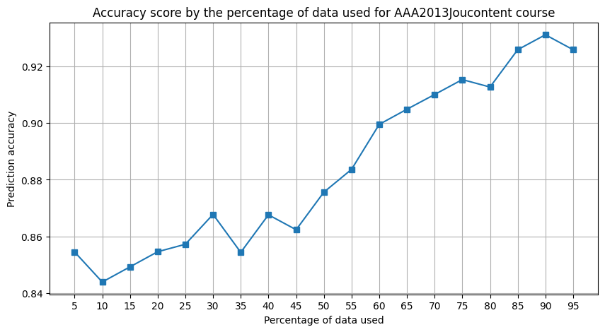
Early dropout prediction

The earlier we can accurately forecast student dropout, the more beneficial the approach becomes by affording MOOC instructors extra time for intervention. As in the work of Lui et al., we compare the predictive accuracy of the TimeSeriesForest classification using incrementally larger fractions of the original data. We start with a 5 percent dataset and iteratively add 5 percent increments to assess how prediction accuracy evolves.

%%capture -ns time_series_classification_for_dropout_prediction a_scores c_scores
def get_score_by_slice(index_slice) -> Iterator[float]:
    """Computes accuracy prediction scores for the given `index_slice`."""
    y = click_stream.loc[index_slice, "final_result"].values
    for i in range(5, 100, 5):
        estimator = TimeSeriesForestClassifier(n_estimators=500)
        limit = round((click_stream.columns.shape[0] - 1) * i / 100)
        X = click_stream.loc[index_slice, click_stream.columns[:limit]].values
        yield np.mean(
            cross_val_score(estimator, X, y, cv=10, scoring="accuracy", n_jobs=-1)
        )


a_scores = pd.Series(
    list(get_score_by_slice(("AAA", "2013J", slice(None), "oucontent"))),
    index=range(5, 100, 5),
)
c_scores = pd.Series(
    list(get_score_by_slice(("CCC", "2014J", slice(None), "resource"))),
    index=range(5, 100, 5),
)
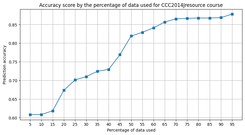
for scores, name in [(a_scores, "AAA2013Joucontent"), (c_scores, "CCC2014Jresource")]:
    scores.plot(
        title=f"Accuracy score by the percentage of data used for {name} course",
        xlabel="Percentage of data used",
        ylabel="Prediction accuracy",
        xticks=range(5, 100, 5),
        figsize=(10, 5),
        grid=True,
        marker="s",
    )
    plt.show()